Polygon Tutorial

h3-py can convert between sets of cells and GeoJSON-like polygon and multipolygon shapes.

We use the abstract base class H3Shape and its concrete child classes H3Poly and H3MultiPoly to represent these shapes. Any references or function names that use “H3Shape” will apply to both H3Poly and H3MultiPoly objects.

h3-py is also compatible with Python objects that implement __geo_interface__ (https://gist.github.com/sgillies/2217756), making it easy to interface with other Python geospatial libraries. We’ll refer to any such object as a “geo” or “geo object”.

H3Poly and H3MultiPoly both implement __geo_interface__ (making them geo objects themselves), and can be created from other geo objects, like Shapely’s Polygon or MultiPolygon objects that occur when using geopandas.

Below, we’ll explain the h3-py API for working with these shapes, and how the library interacts with other Python geospatial libraries.

To start, we’ll import relevant libraries, and define some plotting helper functions to visualize the shapes we’re dealing with.

import h3

import geopandas
import geodatasets
import contextily as cx
import matplotlib.pyplot as plt

def plot_df(df, column=None, ax=None):
    'Plot based on the `geometry` column of a GeoPandas dataframe'
    df = df.copy()
    df = df.to_crs(epsg=3857) # web mercator

    if ax is None:
        fig, ax = plt.subplots(figsize=(8,8))
    ax.get_xaxis().set_visible(False)
    ax.get_yaxis().set_visible(False)
    
    df.plot(
        ax=ax,
        alpha=0.5, edgecolor='k',
        column=column, categorical=True,
        legend=True, legend_kwds={'loc': 'upper left'}, 
    )
    cx.add_basemap(ax, crs=df.crs, source=cx.providers.CartoDB.Positron)

def plot_shape(shape, ax=None):
    df = geopandas.GeoDataFrame({'geometry': [shape]}, crs='EPSG:4326')
    plot_df(df, ax=ax)

def plot_cells(cells, ax=None):
    shape = h3.cells_to_h3shape(cells)
    plot_shape(shape, ax=ax)

def plot_shape_and_cells(shape, res=9):
    fig, axs = plt.subplots(1,2, figsize=(10,5), sharex=True, sharey=True)
    plot_shape(shape, ax=axs[0])
    plot_cells(h3.h3shape_to_cells(shape, res), ax=axs[1])
    fig.tight_layout()

H3Poly

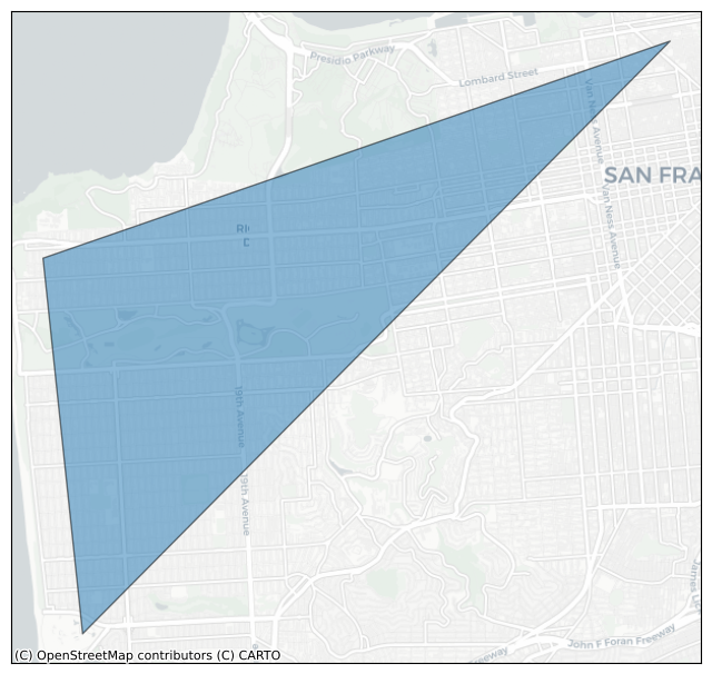
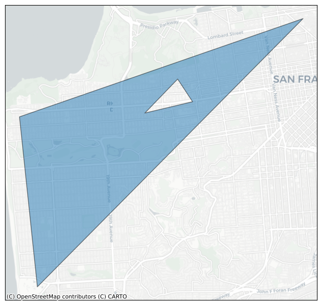
We can create a simple H3Poly object by providing a list of the latitude/longitude pairs that describe its exterior. Optionally, holes can be added to the polygon by appending additional lat/lng lists do describe them.

outer = [
    (37.804, -122.412),
    (37.778, -122.507),
    (37.733, -122.501)
]

poly = h3.H3Poly(outer)
print(poly)
plot_shape(poly)

<H3Poly: [3]>

hole1 = [
    (37.782, -122.449),
    (37.779, -122.465),
    (37.788, -122.454),
]

poly = h3.H3Poly(outer, hole1)
print(poly)
plot_shape(poly)

<H3Poly: [3/(3,)]>

hole2 = [
    (37.771, -122.484),
    (37.761, -122.481),
    (37.758, -122.494),
    (37.769, -122.496),
]

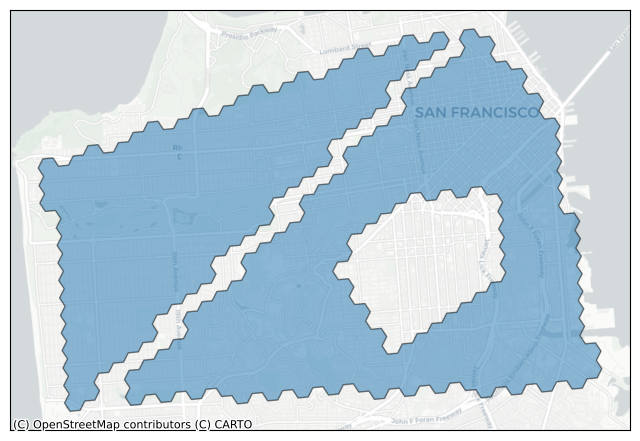
poly = h3.H3Poly(outer, hole1, hole2)
print(poly)
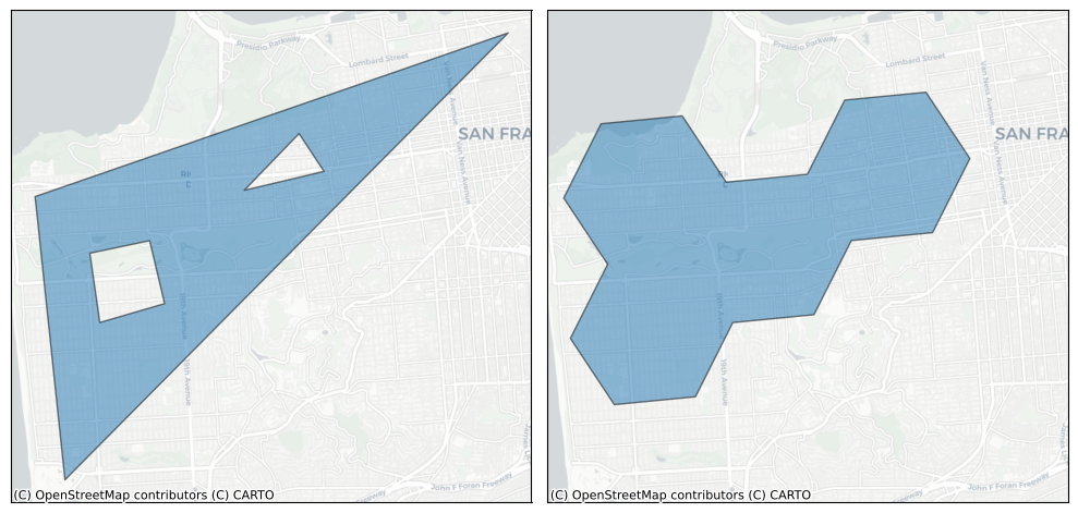
plot_shape(poly)

<H3Poly: [3/(3, 4)]>

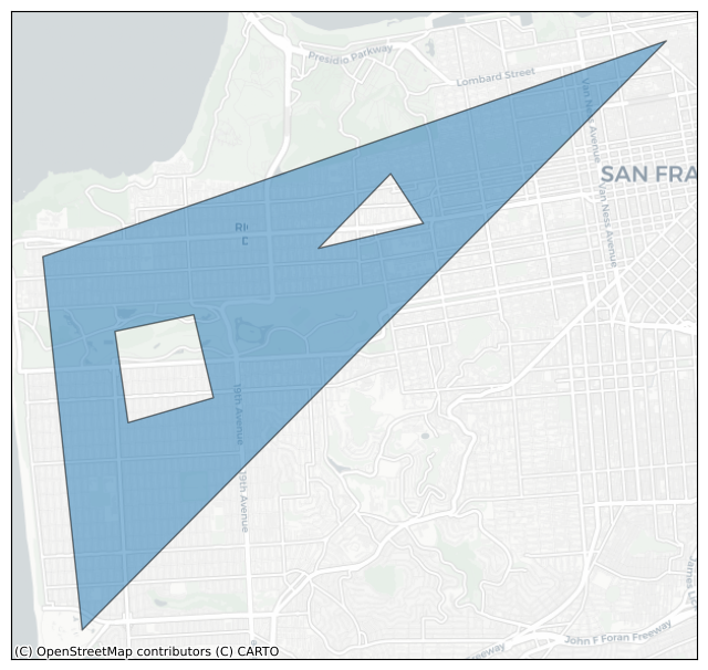
String representation and attributes

The H3Poly string representation given by its __repr__ shows the number of vertices in the outer loop of the polygon, followed by the number of vertices in each hole.

A representation like

<H3Poly: [3/(3, 4)]>

denotes a polygon whose outer boundary consists of 3 vertices and which has 2 holes, with 3 and 4 vertices respectively.

We can access the coordinates describing the polygon through the attributes:

• H3Poly.outer gives the list of lat/lng points making up the outer loop of the polygon.

• H3Poly.holes gives each of the lists of lat/lng points making up the holes of the polygon.

poly = h3.H3Poly(outer, hole1, hole2)
poly

<H3Poly: [3/(3, 4)]>

poly.outer

((37.804, -122.412), (37.778, -122.507), (37.733, -122.501))

poly.holes

([(37.782, -122.449), (37.779, -122.465), (37.788, -122.454)],
 [(37.771, -122.484),
  (37.761, -122.481),
  (37.758, -122.494),
  (37.769, -122.496)])

__geo_interface__

H3Poly.__geo_interface__ gives a GeoJSON representation of the polygon as described in https://gist.github.com/sgillies/2217756

Note the differences in this representation: Points are given in lng/lat order (but the H3Poly constructor expects lat/lng order), and the last vertex repeats the first.

d = poly.__geo_interface__
d

{'type': 'Polygon',
 'coordinates': (((-122.412, 37.804),
   (-122.507, 37.778),
   (-122.501, 37.733),
   (-122.412, 37.804)),
  ((-122.449, 37.782),
   (-122.465, 37.779),
   (-122.454, 37.788),
   (-122.449, 37.782)),
  ((-122.484, 37.771),
   (-122.481, 37.761),
   (-122.494, 37.758),
   (-122.496, 37.769),
   (-122.484, 37.771)))}

print(poly.outer)
print(poly.holes)

((37.804, -122.412), (37.778, -122.507), (37.733, -122.501))
([(37.782, -122.449), (37.779, -122.465), (37.788, -122.454)], [(37.771, -122.484), (37.761, -122.481), (37.758, -122.494), (37.769, -122.496)])

We can create an H3Poly object from a GeoJSON-like dictionary or an object that implements __geo_interface__ using h3.geo_to_h3shape().

h3.geo_to_h3shape(d)

<H3Poly: [3/(3, 4)]>

class MockGeo:
    def __init__(self, d):
        self.d = d

    @property
    def __geo_interface__(self):
        return self.d

geo = MockGeo(d)
h3.geo_to_h3shape(geo)

<H3Poly: [3/(3, 4)]>

Also note that H3Poly.__geo_interface__ is equivalent to calling h3.h3shape_to_geo() on an H3Poly object.

poly.__geo_interface__ == h3.h3shape_to_geo(poly)

True

Polygon to cells

We can get all the H3 cells whose centroids fall within an H3Poly by using h3.h3shape_to_cells() and specifying the resolution.

h3.h3shape_to_cells(poly, res=7)

['872830958ffffff', '87283095bffffff', '87283095affffff', '872830829ffffff']

We’ll use a helper function to show a few different resolutions.

plot_shape_and_cells(poly, 7)

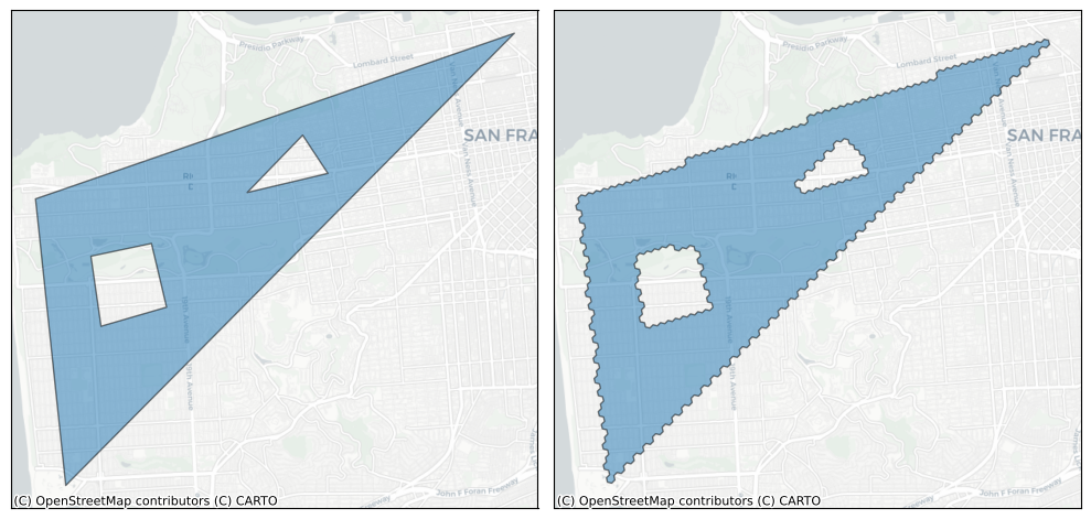
plot_shape_and_cells(poly, 9)

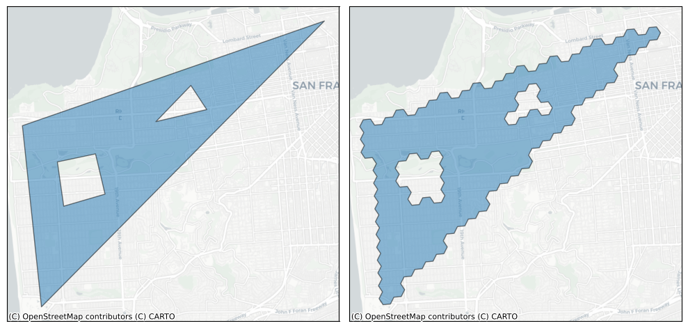
plot_shape_and_cells(poly, 10)

H3 Polygons don’t need to follow the right-hand rule

H3Poly objects do not need to follow the “right-hand rule”, unlike GeoJSON Polygons. The right-hand rule requires that vertices in outer loops are listed in counterclockwise order and holes are listed in clockwise order. h3-py accepts loops in any order and will usually interpret them as the user intended, for example, converting to sets of cells. However, h3-py won’t re-order your loops to conform to the right-hand rule, so be careful if you’re using __geo_interface__ to plot them.

Obeying the right-hand rule is only a concern when creating H3Poly objects from external input; H3Poly or H3MultiPoly objects created through h3.cells_to_shape() will respect the right-hand rule.

For example, if we reverse the order of one of the holes in our example polygon above, the hole won’t be rendered correctly, but the conversion to cells will remain unchanged.

# Respects right-hand rule
poly = h3.H3Poly(outer, hole1, hole2)
plot_shape_and_cells(poly, res=10)

# Does not respect right-hand-rule; second hole is reversed
# Conversion to cells still works, tho!
poly = h3.H3Poly(outer, hole1[::-1], hole2)
plot_shape_and_cells(poly, res=10)

# Does not respect right-hand-rule; outer loop and second hole are both reversed
# Conversion to cells still works, tho!
poly = h3.H3Poly(outer[::-1], hole1[::-1], hole2)
plot_shape_and_cells(poly, res=10)

H3MultiPoly

An H3MultiPoly can be created from H3Poly objects. The string representation of the H3MultiPoly gives the number of vertices in the outer loop of each H3Poly, along with the number of vertices in each hole (if there are any).

For example <H3MultiPoly: [3], [4/(5,)]> represents an H3MultiPoly consisting of two H3Poly polygons:

• the first polygon has 3 outer vertices and no holes

• the second polygon has 4 outer vertices and 1 hole with 5 vertices

poly1 = h3.H3Poly([(37.804, -122.412), (37.778, -122.507), (37.733, -122.501)])
poly2 = h3.H3Poly(
    [(37.803, -122.408), (37.736, -122.491), (37.738, -122.380), (37.787, -122.39)],
    [(37.760, -122.441), (37.772, -122.427), (37.773, -122.404), (37.758, -122.401), (37.745, -122.428)]
)
mpoly = h3.H3MultiPoly(poly1, poly2)

print(poly1)
print(poly2)
print(mpoly)

<H3Poly: [3]>
<H3Poly: [4/(5,)]>
<H3MultiPoly: [3], [4/(5,)]>

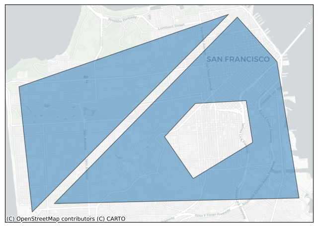
plot_shape(mpoly)

MultiPolygon to cells

h3.h3shape_to_cells() works on both H3MultiPoly and H3Poly objects (both are subclasses of H3Shape).

cells = h3.h3shape_to_cells(mpoly, res=9)
plot_cells(cells)

H3MultiPoly affordances

• Calling len() on an H3MultiPoly gives the number of polygons

• You can iterate through a H3MultiPoly, with the elements being the underlying H3Polys

len(mpoly)

2

for p in mpoly:
    print(p)

<H3Poly: [3]>
<H3Poly: [4/(5,)]>

list(mpoly)

[<H3Poly: [3]>, <H3Poly: [4/(5,)]>]

__geo_interface__

H3MultiPoly implements __geo_interface__, and H3MultiPoly objects can also be created through h3.geo_to_h3shape().

d = mpoly.__geo_interface__
d

{'type': 'MultiPolygon',
 'coordinates': ((((-122.412, 37.804),
    (-122.507, 37.778),
    (-122.501, 37.733),
    (-122.412, 37.804)),),
  (((-122.408, 37.803),
    (-122.491, 37.736),
    (-122.38, 37.738),
    (-122.39, 37.787),
    (-122.408, 37.803)),
   ((-122.441, 37.76),
    (-122.427, 37.772),
    (-122.404, 37.773),
    (-122.401, 37.758),
    (-122.428, 37.745),
    (-122.441, 37.76))))}

geo = MockGeo(d)
h3.geo_to_h3shape(geo)

<H3MultiPoly: [3], [4/(5,)]>

Cells to H3Poly or H3MultiPoly

If you have a set of H3 cells that you would like to visualize, you may want to convert them to H3Poly or H3MultiPoly objects using h3.cells_to_h3shape() and then use __geo_interface__ to get their GeoJSON representation. Or you could use h3.cells_to_geo() to get the GeoJSON dictionary directly.

h = h3.latlng_to_cell(37.804, -122.412, res=9)
cells = h3.grid_ring(h, 2)
cells

['89283082b57ffff',
 '89283082b43ffff',
 '89283082b4bffff',
 '89283080cb3ffff',
 '89283080ca3ffff',
 '89283080ca7ffff',
 '89283080dd3ffff',
 '89283082b6fffff',
 '89283082b67ffff',
 '89283082b77ffff',
 '89283082b0fffff',
 '89283082b0bffff']

plot_cells(cells)

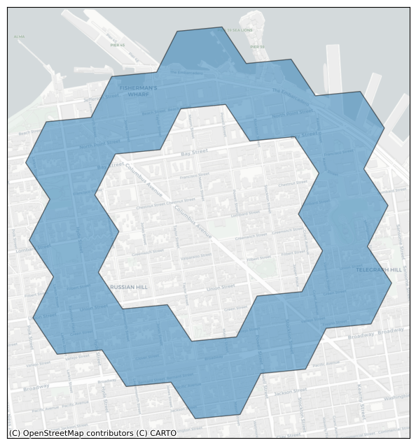
h3.cells_to_h3shape(cells)

<H3Poly: [30/(18,)]>

str(h3.cells_to_geo(cells))[:200]

"{'type': 'Polygon', 'coordinates': (((-122.40793197004145, 37.79671486372511), (-122.40686017324762, 37.79839728727325), (-122.40452852636689, 37.79857529774559), (-122.40345663168632, 37.800257690919"

API Summary

"Geo object" <-> H3Shape <-> H3 cells

“Geo objects” are any Python object that implements __geo_interface__. This is a widely used standard in geospatial Python and is used by libraries like geopandas and Shapely.

H3Shape is an abstract class implemented by H3Poly and H3MultiPoly, each of which implement __geo_interface__ and can be created from external “Geo objects”:

• geo_to_h3shape()

• h3shape_to_geo()

H3Shape objects can be converted to and from sets of H3 cells:

• h3shape_to_cells()

• cells_to_h3shape()

For convience, we provide functions that hide the intermediate H3Shape representation:

• geo_to_cells()

• cells_to_geo()

Equivalance notes

Note that if an object a is an H3Shape then the following two expressions are equivalent:

• h3shape_to_geo(a)

• a.__geo_interface__

Also note that if a is an H3Shape, then a “passes through” geo_to_h3shape():

geo_to_h3shape(a) == a

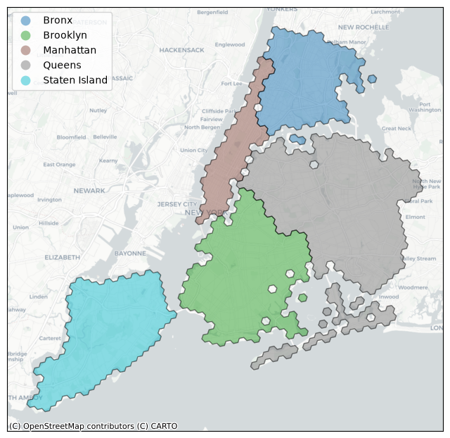
Interfacing with GeoPandas and other libraries

The __geo_interface__ compatibility allows h3-py to work with geopandas and other geospatial libraries easily.

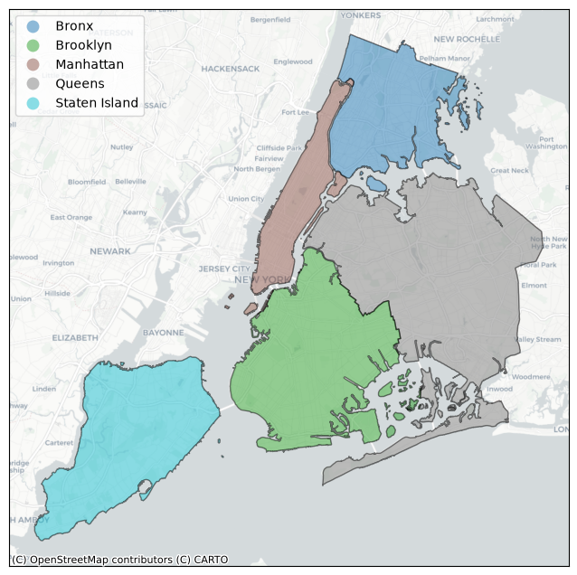
To demonstrate, we start with a GeoPandas GeoDataFrame describing the five New York City boroughs.

df = geopandas.read_file(geodatasets.get_path('nybb'))
df

Downloading file 'nybb_16a.zip' from 'https://www.nyc.gov/assets/planning/download/zip/data-maps/open-data/nybb_16a.zip' to '/home/runner/.cache/geodatasets'.

Extracting 'nybb_16a/nybb.shp' from '/home/runner/.cache/geodatasets/nybb_16a.zip' to '/home/runner/.cache/geodatasets/nybb_16a.zip.unzip'

Extracting 'nybb_16a/nybb.shx' from '/home/runner/.cache/geodatasets/nybb_16a.zip' to '/home/runner/.cache/geodatasets/nybb_16a.zip.unzip'

Extracting 'nybb_16a/nybb.dbf' from '/home/runner/.cache/geodatasets/nybb_16a.zip' to '/home/runner/.cache/geodatasets/nybb_16a.zip.unzip'

Extracting 'nybb_16a/nybb.prj' from '/home/runner/.cache/geodatasets/nybb_16a.zip' to '/home/runner/.cache/geodatasets/nybb_16a.zip.unzip'

	BoroCode	BoroName	Shape_Leng	Shape_Area	geometry
0	5	Staten Island	330470.010332	1.623820e+09	MULTIPOLYGON (((970217.022 145643.332, 970227....
1	4	Queens	896344.047763	3.045213e+09	MULTIPOLYGON (((1029606.077 156073.814, 102957...
2	3	Brooklyn	741080.523166	1.937479e+09	MULTIPOLYGON (((1021176.479 151374.797, 102100...
3	1	Manhattan	359299.096471	6.364715e+08	MULTIPOLYGON (((981219.056 188655.316, 980940....
4	2	Bronx	464392.991824	1.186925e+09	MULTIPOLYGON (((1012821.806 229228.265, 101278...

plot_df(df, column='BoroName')

Use a compatible CRS before applying H3 functions

The function h3.geo_to_cells(geo, res) takes some “geo object” that implements __geo_interface__ (https://gist.github.com/sgillies/2217756) — like a Shapely Polygon or MultiPolygon — and converts it to the set of cells whose centroids are contained in geo.

Common Pitfall: Be careful about what CRS you are using. h3-py expects coordinates as latitude-longitude pairs. The CRS of the current dataframe (EPSG:2263) gives coordinates in feet! You should first convert the data to something compatible. A common choice is EPSG:4326/WGS84. You’ll get incorrect results if you apply h3.geo_to_cells without converting.

# Original CRS
df.crs

<Projected CRS: EPSG:2263>
Name: NAD83 / New York Long Island (ftUS)
Axis Info [cartesian]:
- X[east]: Easting (US survey foot)
- Y[north]: Northing (US survey foot)
Area of Use:
- name: United States (USA) - New York - counties of Bronx; Kings; Nassau; New York; Queens; Richmond; Suffolk.
- bounds: (-74.26, 40.47, -71.8, 41.3)
Coordinate Operation:
- name: SPCS83 New York Long Island zone (US Survey feet)
- method: Lambert Conic Conformal (2SP)
Datum: North American Datum 1983
- Ellipsoid: GRS 1980
- Prime Meridian: Greenwich

df.geometry[0]

# Converting to EPSG:4326/WGS84
df = df.to_crs(epsg=4326)
df.crs

<Geographic 2D CRS: EPSG:4326>
Name: WGS 84
Axis Info [ellipsoidal]:
- Lat[north]: Geodetic latitude (degree)
- Lon[east]: Geodetic longitude (degree)
Area of Use:
- name: World.
- bounds: (-180.0, -90.0, 180.0, 90.0)
Datum: World Geodetic System 1984 ensemble
- Ellipsoid: WGS 84
- Prime Meridian: Greenwich

# Note that the `geometry` column now has coordinates in degrees
df

	BoroCode	BoroName	Shape_Leng	Shape_Area	geometry
0	5	Staten Island	330470.010332	1.623820e+09	MULTIPOLYGON (((-74.05051 40.56642, -74.05047 ...
1	4	Queens	896344.047763	3.045213e+09	MULTIPOLYGON (((-73.83668 40.59495, -73.83678 ...
2	3	Brooklyn	741080.523166	1.937479e+09	MULTIPOLYGON (((-73.86706 40.58209, -73.86769 ...
3	1	Manhattan	359299.096471	6.364715e+08	MULTIPOLYGON (((-74.01093 40.68449, -74.01193 ...
4	2	Bronx	464392.991824	1.186925e+09	MULTIPOLYGON (((-73.89681 40.79581, -73.89694 ...

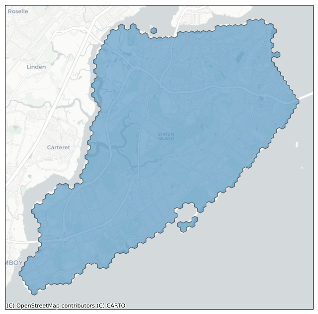
Converting a geo to H3 cells

First, we select one of the boroughs and get the Shapely MultiPolygon describing it.

geo = df.geometry[0]
type(geo)

shapely.geometry.multipolygon.MultiPolygon

Note that Shapely MultiPolygon objects implement __geo_interface__, so we can use h3.geo_to_cells() to get the associated set of H3 cells at various resolutions.

h3.geo_to_cells(geo, res=6)

['862a1062fffffff', '862a10627ffffff', '862a1060fffffff', '862a10607ffffff']

plot_cells(h3.geo_to_cells(geo, res=9))

Converting all geos in a GeoDataFrame to cells

We can apply geo_to_cells() to each of the Shapely geometries in the df.geometry column.

cell_column = df.geometry.apply(lambda x: h3.geo_to_cells(x, res=8))
cell_column

0    [882a106353fffff, 882a106253fffff, 882a107505f...
1    [882a103917fffff, 882a103825fffff, 882a10391df...
2    [882a1076d9fffff, 882a103929fffff, 882a107627f...
3    [882a100d0dfffff, 882a100f2dfffff, 882a100f67f...
4    [882a100f5dfffff, 882a100f43fffff, 882a100007f...
Name: geometry, dtype: object

Converting cells to “geo objects”

If we assign df.geometry = cell_column we’ll get an error because the geometry column of a geopandas.GeoDataFrame must contain valid geometry objects. We can obtain compatible objects by converting the cells to H3Shape by applying h3.cells_to_h3shape().

(Note that, unfortunately, Pandas has some logic to identify iterable members of a series and then renders a tuple of the elements, rather than our preferred H3MultiPoly.__repr__ representation.)

shape_column = cell_column.apply(h3.cells_to_h3shape)
shape_column

0                                      <H3Poly: [132]>
1    (<H3Poly: [178/(6,)]>, <H3Poly: [66/(6,)]>, <H...
2           (<H3Poly: [166/(6, 6, 6)]>, <H3Poly: [6]>)
3                                      <H3Poly: [120]>
4     (<H3Poly: [120]>, <H3Poly: [10]>, <H3Poly: [6]>)
Name: geometry, dtype: object

Note that the column now consists of H3Poly and H3MultiPoly objects.

shape_column[0]

<H3Poly: [132]>

shape_column[1]

<H3MultiPoly: [178/(6,)], [66/(6,)], [22], [30], [10], [6], [6]>

Now, if we assign df.geometry = shape_column, our H3Shape objects will automatically be converted to Shapely Polygon and MultiPolygon objects via __geo_interface__.

df.geometry = shape_column
df.geometry

0    POLYGON ((-74.13326 40.54427, -74.12885 40.540...
1    MULTIPOLYGON (((-73.81285 40.64264, -73.80846 ...
2    MULTIPOLYGON (((-74.01307 40.68399, -74.01503 ...
3    POLYGON ((-74.00964 40.70522, -74.00326 40.706...
4    MULTIPOLYGON (((-73.78392 40.85395, -73.78833 ...
Name: geometry, dtype: geometry

type(df.geometry[0])

shapely.geometry.polygon.Polygon

Visualizing H3 cells

We took some Shapely geometry objects, converted them to H3 cells, and converted those back to Shapely geometry objects in a geopandas.GeoDataFrame.

We can visualize the results with our helper function.

plot_df(df, column='BoroName')