Decompose Prediction

In this section, we will demonstrate how to visualize

• time series forecasting

• predicted components

by using the plotting utilities that come with the Orbit package.

%matplotlib inline

import pandas as pd
import numpy as np
import orbit
from orbit.models.dlt import DLTMAP, DLTFull
from orbit.diagnostics.plot import plot_predicted_data,plot_predicted_components
from orbit.utils.dataset import load_iclaims

import warnings
warnings.filterwarnings('ignore')

assert orbit.__version__ == '1.0.12'

# load log-transformed data
df = load_iclaims()
train_df = df[df['week'] < '2017-01-01']
test_df = df[df['week'] >= '2017-01-01']

response_col = 'claims'
date_col = 'week'
regressor_col = ['trend.unemploy', 'trend.filling', 'trend.job']

Fit a model

Here we use the DLTFull model as example.

dlt = DLTFull(
    response_col=response_col,
    regressor_col=regressor_col,
    date_col=date_col,
    seasonality=52,
    prediction_percentiles=[5, 95],
)

dlt.fit(train_df)

WARNING:pystan:Maximum (flat) parameter count (1000) exceeded: skipping diagnostic tests for n_eff and Rhat.
To run all diagnostics call pystan.check_hmc_diagnostics(fit)

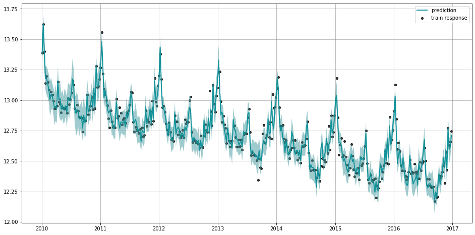
Plot Predictions

First, we do the prediction on the training data before the year 2017.

predicted_df = dlt.predict(df=train_df, decompose=True)

_ = plot_predicted_data(train_df, predicted_df,
                        date_col=dlt.date_col, actual_col=dlt.response_col)

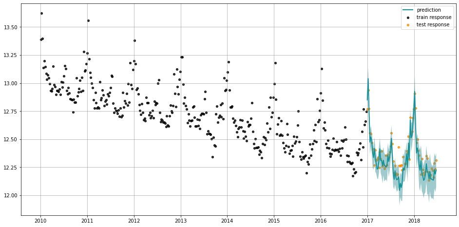
Next, we do the predictions on the test data after the year 2017. This plot is useful to help check the overall model performance on the out-of-sample period.

predicted_df = dlt.predict(df=test_df, decompose=True)

_ = plot_predicted_data(training_actual_df=train_df, predicted_df=predicted_df,
                        date_col=dlt.date_col, actual_col=dlt.response_col,
                        test_actual_df=test_df)

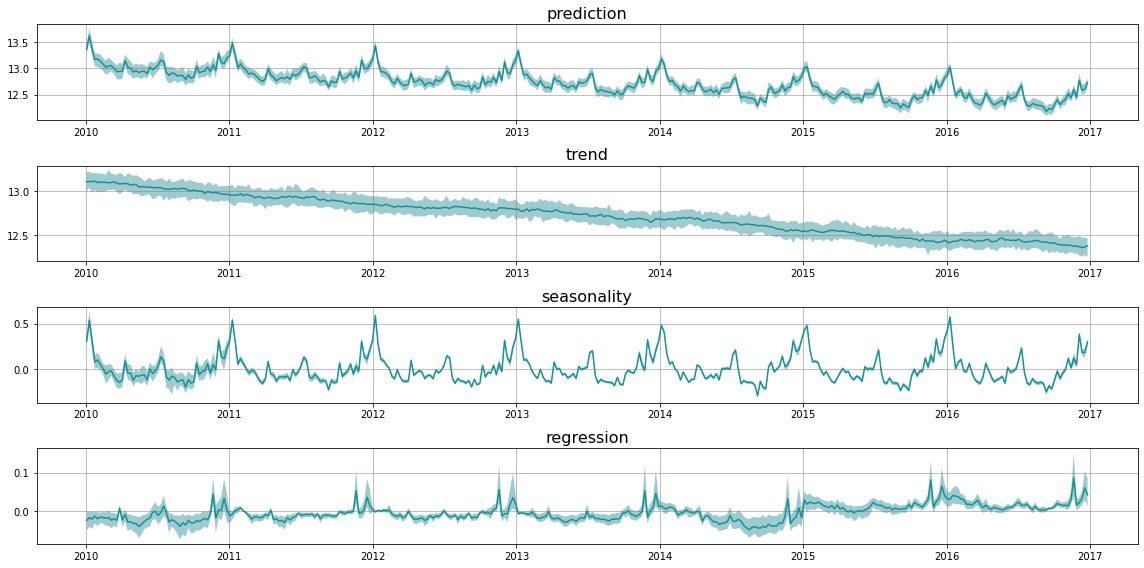
Plot Predicted Components

plot_predicted_components is the utility to plot each component separately. This is useful when one wants to look into the model prediction results and inspect each component separately.

predicted_df = dlt.predict(df=train_df, decompose=True)

_ = plot_predicted_components(predicted_df, date_col)

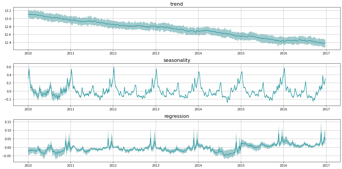
One can use plot_components to have more componets to be plotted if they are available in the supplied predicted_df.

_ = plot_predicted_components(predicted_df, date_col,
                              plot_components=['prediction', 'trend', 'seasonality', 'regression'])