Quick Start
In this session, we will explore:
a forecast task on iclaims dataset
a simple Bayesian ETS Model using
PyStantools to visualize the forecast
Load Library
[1]:
%matplotlib inline
import orbit
from orbit.utils.dataset import load_iclaims
from orbit.models.dlt import ETSFull
from orbit.diagnostics.plot import plot_predicted_data
[2]:
assert orbit.__version__ == '1.0.12'
Data
The iclaims data contains the weekly initial claims for US unemployment benefits against a few related google trend queries (unemploy, filling and job)from Jan 2010 - June 2018. This aims to demo a similar dataset from the Bayesian Structural Time Series (BSTS) model (Scott and Varian 2014).
Number of claims are obtained from Federal Reserve Bank of St. Louis while regressors such as google queries are obtained through Google Trends API.
Note: Both the response and regressors are transformed by log in order to illustrate a multiplicative model. We will continue to use this dataset in some subsequent sections.
[3]:
# load data
df = load_iclaims()
date_col = 'week'
response_col = 'claims'
df.dtypes
[3]:
week              datetime64[ns]
claims                   float64
trend.unemploy           float64
trend.filling            float64
trend.job                float64
sp500                    float64
vix                      float64
dtype: object
[4]:
df.head(5)
[4]:
| week | claims | trend.unemploy | trend.filling | trend.job | sp500 | vix | |
|---|---|---|---|---|---|---|---|
| 0 | 2010-01-03 | 13.386595 | 0.219882 | -0.318452 | 0.117500 | -0.417633 | 0.122654 |
| 1 | 2010-01-10 | 13.624218 | 0.219882 | -0.194838 | 0.168794 | -0.425480 | 0.110445 |
| 2 | 2010-01-17 | 13.398741 | 0.236143 | -0.292477 | 0.117500 | -0.465229 | 0.532339 |
| 3 | 2010-01-24 | 13.137549 | 0.203353 | -0.194838 | 0.106918 | -0.481751 | 0.428645 |
| 4 | 2010-01-31 | 13.196760 | 0.134360 | -0.242466 | 0.074483 | -0.488929 | 0.487404 |
Train / Test Split
[5]:
test_size = 52
train_df = df[:-test_size]
test_df = df[-test_size:]
Forecasting Using Orbit
Orbit aims to provide an intuitive initialize-fit-predict interface for working with forecasting tasks. Under the hood, it is utilizing probabilistic modeling API such as PyStan and Pyro. We first illustrate a Bayesian implementation of Rob Hyndman’s ETS (which stands for Error, Trend, and Seasonality) Model (Hyndman et. al, 2008) using PyStan.
[6]:
dlt = ETSFull(
    response_col=response_col,
    date_col=date_col,
    seasonality=52,
    seed=8888,
)
[7]:
%%time
dlt.fit(df=train_df)
INFO:pystan:COMPILING THE C++ CODE FOR MODEL anon_model_982090c5656030fa038b63e5c383dbff NOW.
WARNING:pystan:n_eff / iter below 0.001 indicates that the effective sample size has likely been overestimated
CPU times: user 1.37 s, sys: 126 ms, total: 1.5 s
Wall time: 45.8 s
[8]:
predicted_df = dlt.predict(df=test_df)
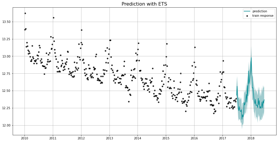
[9]:
_ = plot_predicted_data(train_df, predicted_df, date_col, response_col, title='Prediction with ETS')