Methods of Estimations

In Orbit, we support three methods to estimate model parameters (a.k.a posteriors in Bayesian).

1. Maximum a Posteriori (MAP)

2. Full Bayesian estimation

3. Aggregated posterior estimation

%matplotlib inline

import orbit
from orbit.utils.dataset import load_iclaims
from orbit.models.ets import ETSMAP, ETSFull, ETSAggregated
from orbit.diagnostics.plot import plot_predicted_data

assert orbit.__version__ == '1.0.12'

# load data
df = load_iclaims()
test_size = 52
train_df = df[:-test_size]
test_df = df[-test_size:]
response_col = 'claims'
date_col = 'week'

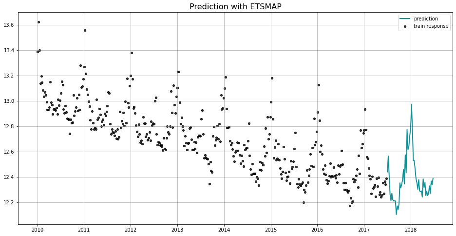
Maximum a Posteriori (MAP)

In general, we use the naming convention of [TheModel]MAP to represent a model class using MAP estimation. You will find the usage of ETSMAP here, and DLTMAP and LGTMAP in the later sections. The advantage of MAP estimation is a faster computational speed. We also provide inference for MAP method, with the caveat that the uncertainty is mainly generated by the noise process and as such we may not observe the uncertainty band from seasonality or other components.

%%time
ets = ETSMAP(
    response_col=response_col,
    date_col=date_col,
    seasonality=52,
    seed=8888,
)
ets.fit(df=train_df)
predicted_df = ets.predict(df=test_df)

CPU times: user 26.5 ms, sys: 8.62 ms, total: 35.1 ms
Wall time: 276 ms

_ = plot_predicted_data(train_df, predicted_df, date_col, response_col, title='Prediction with ETSMAP')

Full Bayesian Estimation

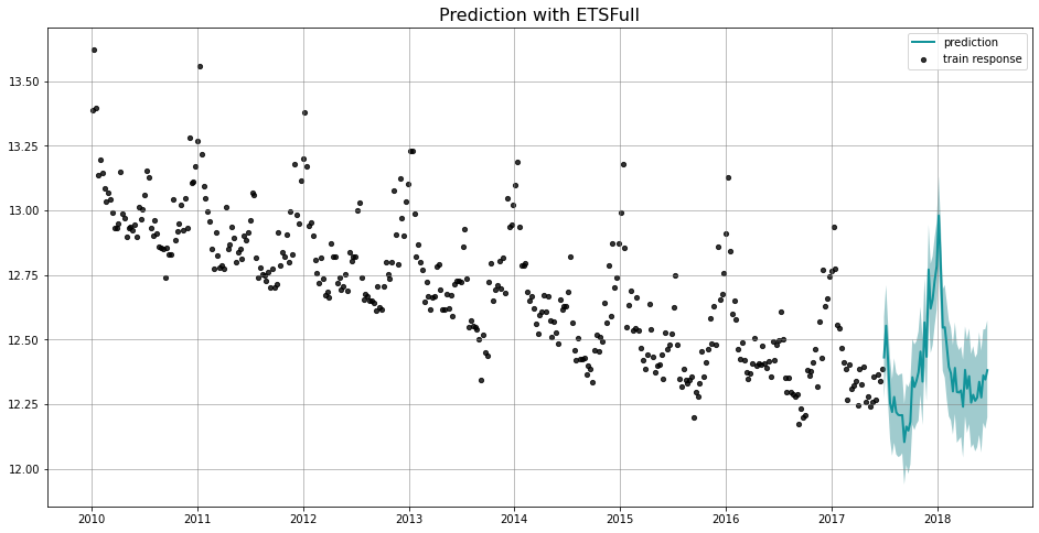
We use the naming convention of [TheModel]Full to represent a model using full Bayesian estimation. For example, you will find the usage of ETSFull here, and DLTFull and LGTFull in the later sections. Compared to MAP, it usually takes longer time to fit a full Bayesian models where No-U-Turn Sampler (NUTS) (Hoffman and Gelman 2011) is carried out under the hood. The advantage is that the inference and estimation are usually more robust.

%%time
ets = ETSFull(
    response_col=response_col,
    date_col=date_col,
    seasonality=52,
    seed=8888,
    num_warmup=400,
    num_sample=400,
)
ets.fit(df=train_df)
predicted_df = ets.predict(df=test_df)

CPU times: user 499 ms, sys: 70.8 ms, total: 570 ms
Wall time: 1.58 s

_ = plot_predicted_data(train_df, predicted_df, date_col, response_col, title='Prediction with ETSFull')

You can also access the posterior samples by the attribute of ._posterior_samples as a dict.

ets._posterior_samples.keys()

odict_keys(['l', 'lev_sm', 'obs_sigma', 's', 'sea_sm', 'lp__'])

Aggregated Posteriors

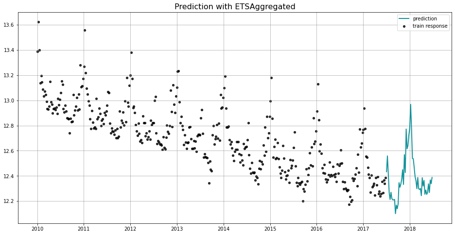
We use the naming convention of [TheModel]Aggregated to represent a model using aggregated posteriors for prediction. For example, you will find the usage of ETSAggregated here, and DLTAggregated and LGTAggregated in later section. Just like the full Bayesian method, it runs through the MCMC algorithm which is NUTS by default. The difference from a full model is that aggregated model first aggregates the posterior samples based on mean or median (via aggregate_method) then does the prediction using the aggreated posterior.

%%time
ets = ETSAggregated(
    response_col=response_col,
    date_col=date_col,
    seasonality=52,
    seed=8888,
)
ets.fit(df=train_df)
predicted_df = ets.predict(df=test_df)

WARNING:pystan:n_eff / iter below 0.001 indicates that the effective sample size has likely been overestimated

CPU times: user 315 ms, sys: 81.4 ms, total: 396 ms
Wall time: 1.7 s

_ = plot_predicted_data(train_df, predicted_df, date_col, response_col, title='Prediction with ETSAggregated')

For users who are interested in the two Orbit refined models – DLT and LGT. There are sections designated to the discussion of the details.