Local Global Trend (LGT)

In this section, we will cover:

• LGT model structure

• difference between DLT and LGT

• syntax to call LGT classes with different estimation methods

LGT stands for Local and Global Trend and is a refined model from Rlgt (Smyl et al., 2019). The main difference is that LGT is an additive form taking log-transformation response as the modeling response. This essentially converts the model into a multicplicative with some advantages (Ng and Wang et al., 2020). However, one drawback of this approach is that negative response values are not allowed due to the existence of the global trend term and because of that we start to deprecate the support of regression of this model.

import pandas as pd
import numpy as np
from orbit.models.lgt import LGTMAP, LGTAggregated, LGTFull
from orbit.diagnostics.plot import plot_predicted_data
from orbit.diagnostics.plot import plot_predicted_components
from orbit.utils.dataset import load_iclaims

Model Structure

\[\begin{split}\begin{align*} y_{t} &= \mu_t + s_t + \epsilon_t \\ \mu_t &= l_{t-1} + \xi_1 b_{t-1} + \xi_2 l_{t-1}^{\lambda}\\ \epsilon_t &~\sim \mathtt{Student}(\nu, 0, \sigma)\\ \sigma &~\sim \mathtt{HalfCauchy}(0, \gamma_0) \end{align*}\end{split}\]

with the update process,

\[\begin{split}\begin{align*} l_t &= \rho_l(y_t - s_t) + (1-\rho_l)l_{t-1}\\ b_t &= \rho_b(l_t - l_{t-1}) + (1-\rho_b)b_{t-1}\\ s_{t+m} &= \rho_s(y_t - l_t ) + (1-\rho_s)s_t \end{align*}\end{split}\]

Unlike DLT model which has a deterministic trend, LGT introduces a hybrid trend where it consists of

• local trend takes on a fraction \(\xi_1\) rather than a damped factor

• global trend is with a auto-regrssive term \(\xi_2\) and a power term \(\lambda\)

We will continue to use the iclaims data with 52 weeks train-test split.

# load data
df = load_iclaims()
# define date and response column
date_col = 'week'
response_col = 'claims'
df.dtypes
test_size = 52
train_df = df[:-test_size]
test_df = df[-test_size:]

LGT Model

In orbit, we have three types of LGT models, LGTMAP, LGTAggregated and LGTFull. Orbit follows a sklearn style model API. We can create an instance of the Orbit class and then call its fit and predict methods.

LGTMAP

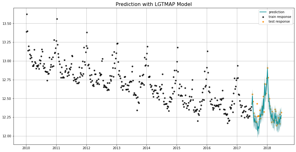
LGTMAP is the model class for MAP (Maximum a Posteriori) estimation.

lgt = LGTMAP(
    response_col=response_col,
    date_col=date_col,
    seasonality=52,
    seed=8888,
)

%%time
lgt.fit(df=train_df)

INFO:pystan:COMPILING THE C++ CODE FOR MODEL anon_model_2af9ff5e07f97061bbe4badb0f8a2e36 NOW.

CPU times: user 1.39 s, sys: 87.2 ms, total: 1.48 s
Wall time: 55.5 s

predicted_df = lgt.predict(df=test_df)

_ = plot_predicted_data(training_actual_df=train_df, predicted_df=predicted_df,
                        date_col=date_col, actual_col=response_col,
                        test_actual_df=test_df, title='Prediction with LGTMAP Model')

LGTFull

LGTFull is the model class for full Bayesian prediction. In full Bayesian prediction, the prediction will be conducted once for each parameter posterior sample, and the final prediction results are aggregated. Prediction will always return the median (aka 50th percentile) along with any additional percentiles that are provided.

lgt = LGTFull(
    response_col=response_col,
    date_col=date_col,
    seasonality=52,
    seed=8888,
)

%%time
lgt.fit(df=train_df)

WARNING:pystan:Maximum (flat) parameter count (1000) exceeded: skipping diagnostic tests for n_eff and Rhat.
To run all diagnostics call pystan.check_hmc_diagnostics(fit)
WARNING:pystan:1 of 100 iterations ended with a divergence (1 %).
WARNING:pystan:Try running with adapt_delta larger than 0.8 to remove the divergences.

CPU times: user 62.4 ms, sys: 63.5 ms, total: 126 ms
Wall time: 6.16 s

predicted_df = lgt.predict(df=test_df)

predicted_df.tail(5)

	week	prediction_5	prediction	prediction_95
47	2018-05-27	12.099949	12.232984	12.330652
48	2018-06-03	12.060341	12.173674	12.293869
49	2018-06-10	12.118473	12.262561	12.408782
50	2018-06-17	12.097858	12.239122	12.341881
51	2018-06-24	12.193468	12.281816	12.383324

_ = plot_predicted_data(training_actual_df=train_df, predicted_df=predicted_df,
                    date_col=lgt.date_col, actual_col=lgt.response_col,
                    test_actual_df=test_df, title='Prediction with LGTFull Model')

LGTAggregated

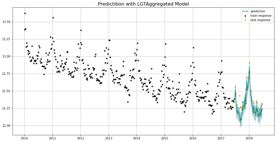
LGTAggregated is the model class for aggregated posterior prediction. In aggregated prediction, the parameter posterior samples are reduced using aggregate_method ({ 'mean', 'median' }) before performing a single prediction.

lgt = LGTAggregated(
    response_col=response_col,
    date_col=date_col,
    seasonality=52,
    seed=8888,
)

%%time
lgt.fit(df=train_df)

WARNING:pystan:Maximum (flat) parameter count (1000) exceeded: skipping diagnostic tests for n_eff and Rhat.
To run all diagnostics call pystan.check_hmc_diagnostics(fit)
WARNING:pystan:1 of 100 iterations ended with a divergence (1 %).
WARNING:pystan:Try running with adapt_delta larger than 0.8 to remove the divergences.

CPU times: user 71.8 ms, sys: 76.5 ms, total: 148 ms
Wall time: 6.38 s

predicted_df = lgt.predict(df=test_df)

predicted_df.tail(5)

	week	prediction_5	prediction	prediction_95
47	2018-05-27	12.091428	12.204437	12.313660
48	2018-06-03	12.031525	12.139519	12.250433
49	2018-06-10	12.124013	12.233509	12.345642
50	2018-06-17	12.090025	12.200898	12.311468
51	2018-06-24	12.138503	12.247008	12.357515

_ = plot_predicted_data(training_actual_df=train_df, predicted_df=predicted_df,
                    date_col=lgt.date_col, actual_col=lgt.response_col,
                    test_actual_df=test_df, title='Predictibon with LGTAggregated Model')

More details for each method are available in the docstrings and also here: https://uber.github.io/orbit/orbit.models.html#module-orbit.models.lgt