Regression with DLT
In this notebook, we want to demonstartate how to use different arguments in DLT to train a model with various regression settings. We continue to use iclaims data for the demo purpose:
regular regression
regression with specific signs and priors for regression coefficients
Finally, we will also use a simulated dataset to illustrate different types of regression penalties:
fixed-ridgeauto-ridgelasso
Generally speaking, regression coefficients are more robust under full Bayesian sampling and estimation. Hence, we will use DTLFull in the session.
[1]:
%matplotlib inline

import matplotlib.pyplot as plt

import orbit
from orbit.utils.dataset import load_iclaims
from orbit.models.dlt import DLTFull, DLTMAP
from orbit.diagnostics.plot import plot_predicted_data
from orbit.constants.palette import QualitativePalette

from pylab import rcParams

rcParams['figure.figsize'] = 14, 8
plt.style.use('fivethirtyeight')
[2]:
assert orbit.__version__ == '1.0.12'
US Weekly Initial Claims
Recall the iclaims dataset by previous section. In order to use this data to nowcast the US unemployment claims during COVID-19 period, we extended the dataset to Jan 2021 and added the S&P 500 (^GSPC) and VIX Index historical data for the same period.
The data is standardized and log-transformed for the model fitting purpose.
[3]:
# load data
df = load_iclaims(end_date='2021-01-03')
date_col = 'week'
response_col = 'claims'
df.dtypes
[3]:
week              datetime64[ns]
claims                   float64
trend.unemploy           float64
trend.filling            float64
trend.job                float64
sp500                    float64
vix                      float64
dtype: object
[4]:
df.head(5)
[4]:
| week | claims | trend.unemploy | trend.filling | trend.job | sp500 | vix | |
|---|---|---|---|---|---|---|---|
| 0 | 2010-01-03 | 13.386595 | 0.016351 | -0.345855 | 0.130569 | -0.543044 | 0.082087 |
| 1 | 2010-01-10 | 13.624218 | 0.016351 | -0.222241 | 0.181862 | -0.550891 | 0.069878 |
| 2 | 2010-01-17 | 13.398741 | 0.032611 | -0.319879 | 0.130569 | -0.590640 | 0.491772 |
| 3 | 2010-01-24 | 13.137549 | -0.000179 | -0.222241 | 0.119987 | -0.607162 | 0.388078 |
| 4 | 2010-01-31 | 13.196760 | -0.069172 | -0.269869 | 0.087552 | -0.614339 | 0.446838 |
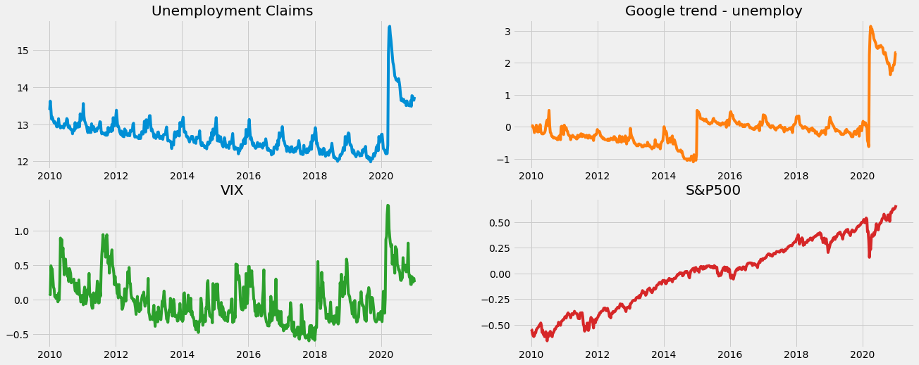
We can see form the plot below, there are seasonlity, trend, and as well as a huge changpoint due the impact of COVID-19.
[5]:
fig, axs = plt.subplots(2, 2,figsize=(20,8))
axs[0, 0].plot(df['week'], df['claims'])
axs[0, 0].set_title('Unemployment Claims')
axs[0, 1].plot(df['week'], df['trend.unemploy'], 'tab:orange')
axs[0, 1].set_title('Google trend - unemploy')
axs[1, 0].plot(df['week'], df['vix'], 'tab:green')
axs[1, 0].set_title('VIX')
axs[1, 1].plot(df['week'], df['sp500'], 'tab:red')
axs[1, 1].set_title('S&P500')
[5]:
Text(0.5, 1.0, 'S&P500')
[6]:
# using relatively updated data
df = df[df['week'] > '2018-01-01'].reset_index(drop=True)
test_size = 26
train_df = df[:-test_size]
test_df = df[-test_size:]
Naive Model
Here we will use DLT models to compare the model performance with vs. without regression.
[7]:
%%time
dlt = DLTFull(
    response_col=response_col,
    date_col=date_col,
    seasonality=52,
    seed=8888,
    num_warmup=4000,
)
dlt.fit(df=train_df)
predicted_df = dlt.predict(df=test_df)
WARNING:pystan:n_eff / iter below 0.001 indicates that the effective sample size has likely been overestimated
WARNING:pystan:Rhat above 1.1 or below 0.9 indicates that the chains very likely have not mixed
CPU times: user 199 ms, sys: 119 ms, total: 318 ms
Wall time: 25.2 s
DLT With Regression
The regressor columns can be supplied via argument regressor_col. Recall the regression formula in DLT:
Let’s use the default where \(\mu_j = 0\) and \(\sigma_j = 1\). In addition, we can set a sign constraint for each coefficient \(\beta_j\). This is can be done by supplying the regressor_sign as a list where elements are in one of followings:
‘=’: \(\beta_j ~\sim \mathcal{N}(0, \sigma_j^2)\) i.e. \(\beta_j \in (-\inf, \inf)\)
‘+’: \(\beta_j ~\sim \mathcal{N}^+(0, \sigma_j^2)\) i.e. \(\beta_j \in [0, \inf)\)
‘-’: \(\beta_j ~\sim \mathcal{N}^-(0, \sigma_j^2)\) i.e. \(\beta_j \in (-\inf, 0]\)
Based on some intuition, it’s reasonable to assume search terms such as “unemployment”, “filling” and VIX index to be positively correlated and stock index such as SP500 to be negatively correlated to the outcome. Then we will leave whatever unsured as a regular regressor.
[8]:
%%time
dlt_reg = DLTFull(
    response_col=response_col,
    date_col=date_col,
    regressor_col=['trend.unemploy', 'trend.filling', 'trend.job', 'sp500', 'vix'],
    regressor_sign=["+", '+', '=', '-', '+'],
    seasonality=52,
    seed=8888,
    num_warmup=4000,
)
dlt_reg.fit(df=train_df)
predicted_df_reg = dlt_reg.predict(test_df)
WARNING:pystan:n_eff / iter below 0.001 indicates that the effective sample size has likely been overestimated
WARNING:pystan:Rhat above 1.1 or below 0.9 indicates that the chains very likely have not mixed
CPU times: user 214 ms, sys: 123 ms, total: 337 ms
Wall time: 20.9 s
The estimated regressor coefficients can be retrieved via .get_regression_coefs().
[9]:
dlt_reg.get_regression_coefs()
[9]:
| regressor | regressor_sign | coefficient | |
|---|---|---|---|
| 0 | trend.unemploy | Positive | 0.868930 |
| 1 | trend.filling | Positive | 0.408123 |
| 2 | vix | Positive | 0.067099 |
| 3 | sp500 | Negative | -0.457451 |
| 4 | trend.job | Regular | 0.007117 |
DLT with Regression and Informative Priors
Assuming users obtain further knowledge on some of the regressors, they could use informative priors (\(\mu\), \(\sigma\)) by replacing the defaults. This can be done via the arguments regressor_beta_prior and regressor_sigma_prior. These two lists should be of the same lenght as regressor_col.
[10]:
dlt_reg_adjust = DLTFull(
    response_col=response_col,
    date_col=date_col,
    regressor_col=['trend.unemploy', 'trend.filling', 'trend.job', 'sp500', 'vix'],
    regressor_sign=["+", '+', '=', '-', '+'],
    regressor_beta_prior=[0.5, 0.25, 0.07, -0.3, 0.03],
    regressor_sigma_prior=[0.1] * 5,
    seasonality=52,
    seed=8888,
    num_warmup=4000,
)
dlt_reg_adjust.fit(df=train_df)
predicted_df_reg_adjust = dlt_reg_adjust.predict(test_df)
WARNING:pystan:n_eff / iter below 0.001 indicates that the effective sample size has likely been overestimated
WARNING:pystan:Rhat above 1.1 or below 0.9 indicates that the chains very likely have not mixed
[11]:
dlt_reg_adjust.get_regression_coefs()
[11]:
| regressor | regressor_sign | coefficient | |
|---|---|---|---|
| 0 | trend.unemploy | Positive | 0.286465 |
| 1 | trend.filling | Positive | 0.256349 |
| 2 | vix | Positive | 0.049923 |
| 3 | sp500 | Negative | -0.300763 |
| 4 | trend.job | Regular | 0.065622 |
Let’s compare the holdout performance by using the built-in function smape() .
[12]:
import numpy as np
from orbit.diagnostics.metrics import smape

# to reverse the log-transformation
def smape_adjusted(x, y):
    x = np.exp(x)
    y = np.exp(y)
    return smape(x, y)

naive_smape = smape_adjusted(predicted_df['prediction'].values, test_df['claims'].values)
reg_smape = smape_adjusted(predicted_df_reg['prediction'].values, test_df['claims'].values)
reg_adjust_smape = smape_adjusted(predicted_df_reg_adjust['prediction'].values, test_df['claims'].values)

print('Naive Model: {:.3f}\nRegression Model: {:.3f}\nRefined Regression Model: {:.3f}'.format(
    naive_smape, reg_smape, reg_adjust_smape
))
Naive Model: 0.205
Regression Model: 0.138
Refined Regression Model: 0.120
Regression on Simulated Dataset
Let’s use a simulated dateset to demonstrate sparse regression.
[13]:
import pandas as pd

from orbit.constants.palette import QualitativePalette
from orbit.utils.simulation import make_trend, make_regression
from orbit.diagnostics.metrics import mse
We have developed a few utilites to generate simulated data. For details, please refer to our API doc. In brief, we are generating observations \(y\) such that
where
Regular Regression
Let’s start with a small number of regressors with \(P=10\) and \(T=100\).
[14]:
NUM_OF_REGRESSORS = 10
SERIES_LEN = 50
SEED = 20210101
# sample some coefficients
COEFS = np.random.default_rng(SEED).uniform(-1, 1, NUM_OF_REGRESSORS)
trend = make_trend(SERIES_LEN, rw_loc=0.01, rw_scale=0.1)
x, regression, coefs = make_regression(series_len=SERIES_LEN, coefs=COEFS)
print(regression.shape, x.shape)
(50,) (50, 10)
[15]:
# combine trend and the regression
y = trend + regression
[16]:
x_cols = [f"x{x}" for x in range(1, NUM_OF_REGRESSORS + 1)]
response_col = "y"
dt_col = "date"
obs_matrix = np.concatenate([y.reshape(-1, 1), x], axis=1)
# make a data frame for orbit inputs
df = pd.DataFrame(obs_matrix, columns=[response_col] + x_cols)
# make some dummy date stamp
dt = pd.date_range(start='2016-01-04', periods=SERIES_LEN, freq="1W")
df['date'] = dt
df.shape
[16]:
(50, 12)
Let’s take a peek on the coefficients.
[17]:
coefs
[17]:
array([ 0.38372743, -0.21084054,  0.5404565 , -0.21864409,  0.85529298,
       -0.83838077, -0.54550632,  0.80367924, -0.74643654, -0.26626975])
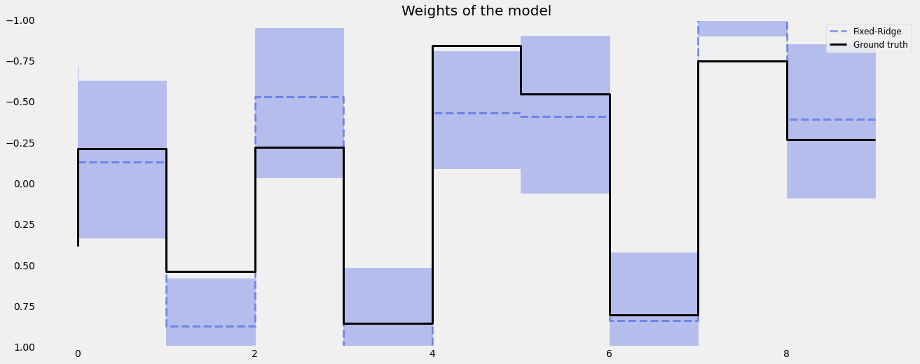
Now, let’s run a regression with the defaults where we have constant regressor_sigma_prior and regression_penalty set as fixed-ridge.
Fixed Ridge Penalty
[18]:
%%time
dlt_fridge = DLTFull(
    response_col=response_col,
    date_col=dt_col,
    regressor_col=x_cols,
    seed=SEED,
    # this is default
    regression_penalty='fixed_ridge',
    # fixing the smoothing parameters to learn regression coefficients more effectively
    level_sm_input=0.01,
    slope_sm_input=0.01,
    num_warmup=4000,
)
dlt_fridge.fit(df=df)
WARNING:pystan:n_eff / iter below 0.001 indicates that the effective sample size has likely been overestimated
WARNING:pystan:Rhat above 1.1 or below 0.9 indicates that the chains very likely have not mixed
CPU times: user 97.6 ms, sys: 90.5 ms, total: 188 ms
Wall time: 4.93 s
[19]:
coef_fridge = np.quantile(dlt_fridge._posterior_samples['beta'], q=[0.05, 0.5, 0.95], axis=0 )
lw=3
idx = np.arange(NUM_OF_REGRESSORS)
plt.figure(figsize=(20, 8))
plt.title("Weights of the model", fontsize=20)
plt.plot(idx, coef_fridge[1], color=QualitativePalette.Line4.value[2], linewidth=lw,  drawstyle='steps', label='Fixed-Ridge', alpha=0.5, linestyle='--')
plt.fill_between(idx, coef_fridge[0], coef_fridge[2], step='pre', alpha=0.3, color=QualitativePalette.Line4.value[2])
plt.plot(coefs, color="black", linewidth=lw,  drawstyle='steps', label="Ground truth")
plt.ylim(1, -1)
plt.legend(prop={'size': 12})
plt.grid()
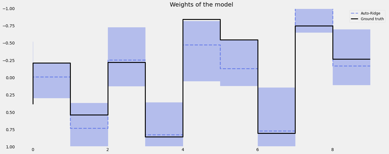
We can also set the regression_penalty to be auto-ridge in case we are sure what to set for the regressor_sigma_prior.
Auto-Ridge Penalty
Instead of using fixed scale in the coefficients prior, a hyperprior can be assigned to them, i.e.
This can be done by setting regression_penalty="auto_ridge" with the argument auto_ridge_scale (default of 0.5) set the hyperprior \(\alpha\). We can also supply stan config such as adapt_delta to reduce divergence. Check the here for details of adapt_delta.
[20]:
%%time
dlt_auto_ridge = DLTFull(
    response_col=response_col,
    date_col=dt_col,
    regressor_col=x_cols,
    seed=SEED,
    # this is default
    regression_penalty='auto_ridge',
    # fixing the smoothing parameters to learn regression coefficients more effectively
    level_sm_input=0.01,
    slope_sm_input=0.01,
    num_warmup=4000,
    # reduce divergence
    stan_mcmc_control={'adapt_delta':0.9},
)
dlt_auto_ridge.fit(df=df)
WARNING:pystan:n_eff / iter below 0.001 indicates that the effective sample size has likely been overestimated
WARNING:pystan:Rhat above 1.1 or below 0.9 indicates that the chains very likely have not mixed
WARNING:pystan:8 of 100 iterations ended with a divergence (8 %).
WARNING:pystan:Try running with adapt_delta larger than 0.9 to remove the divergences.
CPU times: user 110 ms, sys: 102 ms, total: 212 ms
Wall time: 8.98 s
[21]:
coef_auto_ridge = np.quantile(dlt_auto_ridge._posterior_samples['beta'], q=[0.05, 0.5, 0.95], axis=0 )
lw=3
idx = np.arange(NUM_OF_REGRESSORS)
plt.figure(figsize=(20, 8))
plt.title("Weights of the model", fontsize=20)
plt.plot(idx, coef_auto_ridge[1], color=QualitativePalette.Line4.value[2], linewidth=lw,  drawstyle='steps', label='Auto-Ridge', alpha=0.5, linestyle='--')
plt.fill_between(idx, coef_auto_ridge[0], coef_auto_ridge[2], step='pre', alpha=0.3, color=QualitativePalette.Line4.value[2])
plt.plot(coefs, color="black", linewidth=lw,  drawstyle='steps', label="Ground truth")
plt.ylim(1, -1)
plt.legend(prop={'size': 12})
plt.grid()
[22]:
print('Fixed Ridge MSE:{:.3f}\nAuto Ridge MSE:{:.3f}'.format(
    mse(coef_fridge[1], coefs), mse(coef_auto_ridge[1], coefs)
))
Fixed Ridge MSE:0.092
Auto Ridge MSE:0.070
Sparse Regrssion
Now, let’s move to a challenging problem with a much higher \(P\) to \(N\) ratio with a sparsity specified by the parameter relevance=0.5 under the simulation process.
[23]:
NUM_OF_REGRESSORS = 50
SERIES_LEN = 50
SEED = 20210101
COEFS = np.random.default_rng(SEED).uniform(0.3, 0.5, NUM_OF_REGRESSORS)
SIGNS = np.random.default_rng(SEED).choice([1, -1], NUM_OF_REGRESSORS)
# to mimic a either zero or relative observable coefficients
COEFS = COEFS * SIGNS
trend = make_trend(SERIES_LEN, rw_loc=0.01, rw_scale=0.1)
x, regression, coefs = make_regression(series_len=SERIES_LEN, coefs=COEFS, relevance=0.5)
print(regression.shape, x.shape)
(50,) (50, 50)
[24]:
# generated sparsed coefficients
coefs
[24]:
array([ 0.        ,  0.        , -0.45404565,  0.37813559,  0.        ,
        0.        ,  0.        ,  0.48036792, -0.32535635, -0.37337302,
        0.        ,  0.        , -0.37000755,  0.44887456,  0.47082836,
        0.        ,  0.32678039,  0.        ,  0.38932392,  0.40216056,
       -0.34751455, -0.49824576,  0.        , -0.35036047,  0.        ,
        0.        ,  0.        ,  0.        ,  0.3004372 ,  0.        ,
        0.        ,  0.        , -0.49094139,  0.        ,  0.        ,
        0.        , -0.49667658,  0.        ,  0.32336776,  0.        ,
        0.        ,  0.36255583, -0.40961555,  0.        ,  0.44455655,
        0.4449055 ,  0.        ,  0.30064161, -0.46083203,  0.45238241])
[25]:
# combine trend and the regression
y = trend + regression
[26]:
x_cols = [f"x{x}" for x in range(1, NUM_OF_REGRESSORS + 1)]
response_col = "y"
dt_col = "date"
obs_matrix = np.concatenate([y.reshape(-1, 1), x], axis=1)
# make a data frame for orbit inputs
df = pd.DataFrame(obs_matrix, columns=[response_col] + x_cols)
# make some dummy date stamp
dt = pd.date_range(start='2016-01-04', periods=SERIES_LEN, freq="1W")
df['date'] = dt
df.shape
[26]:
(50, 52)
Fixed Ridge Penalty
[27]:
dlt_fridge = DLTFull(
    response_col=response_col,
    date_col=dt_col,
    regressor_col=x_cols,
    seed=SEED,
    level_sm_input=0.01,
    slope_sm_input=0.01,
    num_warmup=8000,
)
dlt_fridge.fit(df=df)
WARNING:pystan:n_eff / iter below 0.001 indicates that the effective sample size has likely been overestimated
WARNING:pystan:Rhat above 1.1 or below 0.9 indicates that the chains very likely have not mixed
[28]:
coef_fridge = np.quantile(dlt_fridge._posterior_samples['beta'], q=[0.05, 0.5, 0.95], axis=0 )
lw=3
idx = np.arange(NUM_OF_REGRESSORS)
plt.figure(figsize=(20, 8))
plt.title("Weights of the model", fontsize=20)
plt.plot(coef_fridge[1], color=QualitativePalette.Line4.value[2], linewidth=lw,  drawstyle='steps', label="Ridge", alpha=0.5, linestyle='--')
plt.fill_between(idx, coef_fridge[0], coef_fridge[2], step='pre', alpha=0.3, color=QualitativePalette.Line4.value[2])
plt.plot(coefs, color="black", linewidth=lw,  drawstyle='steps', label="Ground truth")
plt.legend(prop={'size': 12})
plt.grid()
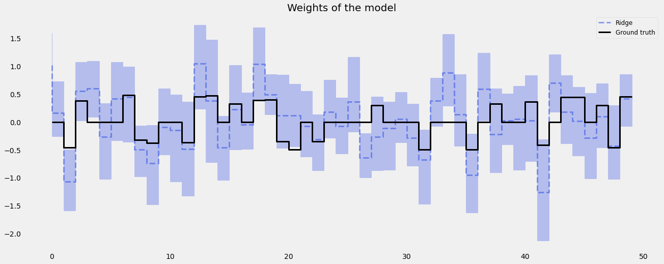
LASSO Penalty
In high \(P\) to \(N\) problems, LASS0 penalty usually shines compared to Ridge penalty.
[29]:
dlt_lasso = DLTFull(
    response_col=response_col,
    date_col=dt_col,
    regressor_col=x_cols,
    seed=SEED,
    regression_penalty='lasso',
    level_sm_input=0.01,
    slope_sm_input=0.01,
    num_warmup=8000,
)
dlt_lasso.fit(df=df)
WARNING:pystan:n_eff / iter below 0.001 indicates that the effective sample size has likely been overestimated
WARNING:pystan:Rhat above 1.1 or below 0.9 indicates that the chains very likely have not mixed
[30]:
coef_lasso = np.quantile(dlt_lasso._posterior_samples['beta'], q=[0.05, 0.5, 0.95], axis=0 )
lw=3
idx = np.arange(NUM_OF_REGRESSORS)
plt.figure(figsize=(20, 8))
plt.title("Weights of the model", fontsize=20)
plt.plot(coef_lasso[1], color=QualitativePalette.Line4.value[2], linewidth=lw,  drawstyle='steps', label="Lasso", alpha=0.5, linestyle='--')
plt.fill_between(idx, coef_lasso[0], coef_lasso[2], step='pre', alpha=0.3, color=QualitativePalette.Line4.value[2])
plt.plot(coefs, color="black", linewidth=lw,  drawstyle='steps', label="Ground truth")
plt.legend(prop={'size': 12})
plt.grid()
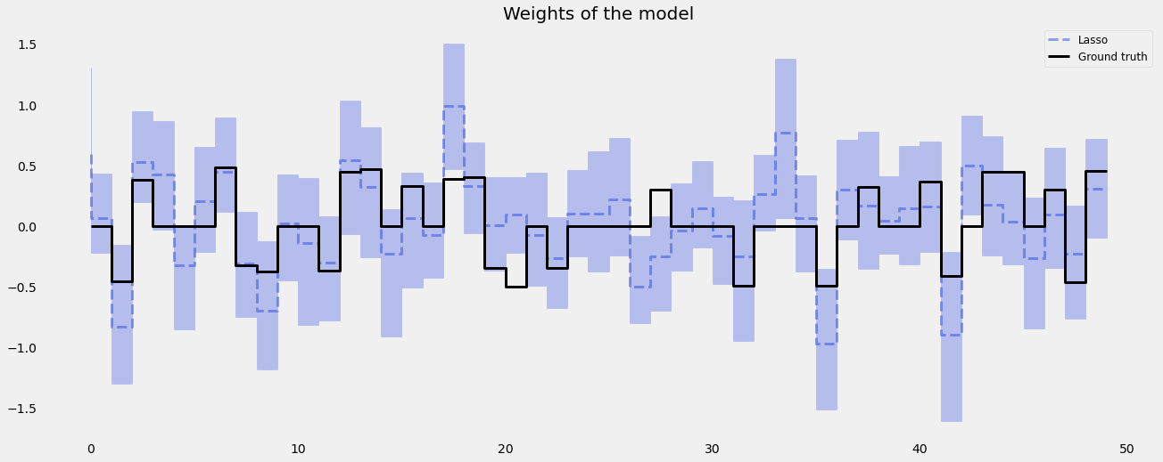
[31]:
print('Fixed Ridge MSE:{:.3f}\nLASSO MSE:{:.3f}'.format(
    mse(coef_fridge[1], coefs), mse(coef_lasso[1], coefs)
))
Fixed Ridge MSE:0.168
LASSO MSE:0.094