Damped Local Trend (DLT)

In this section, we will cover:

• DLT model structure

• DLT global trend configurations

• Adding regressors in DLT

• Other configurations

%matplotlib inline

import orbit
from orbit.models.dlt import DLTMAP
from orbit.diagnostics.plot import plot_predicted_data, plot_predicted_components
from orbit.utils.dataset import load_iclaims

assert orbit.__version__ == '1.0.12'

Model Structure

DLT is one of the main exponential smoothing models we support in orbit. Performance is benchmarked with M3 monthly, M4 weekly dataset and some Uber internal dataset (Ng and Wang et al., 2020). The model is a fusion between the classical ETS (Hyndman et. al., 2008)) with some refinement leveraging ideas from Rlgt (Smyl et al., 2019). The model has a structural forecast equations

\[\begin{split}\begin{align*} y_t &=\mu_t + s_t + r_t + \epsilon_t \\ \mu_t &=g_t + l_{t-1} + \theta{b_{t-1}} \\ \epsilon_t &~\sim \mathtt{Student}(\nu, 0, \sigma)\\ \sigma &~\sim \mathtt{HalfCauchy}(0, \gamma_0) \end{align*}\end{split}\]

with the update process

\[\begin{split}\begin{align*} g_t &= D(t)\\ l_t &= \rho_l(y_t - g_{t} - s_t - r_t) + (1-\rho_l)(l_{t-1} + \theta b_{t-1})\\ b_t &= \rho_b(l_t - l_{t-1}) + (1-\rho_b)\theta b_{t-1}\\ s_{t+m} &= \rho_s(y_t - l_t - r_t) + (1-\rho_s)s_t\\ r_t &= \Sigma_{j}\beta_j x_{jt} \end{align*}\end{split}\]

One important point is that using \(y_t\) as a log-transformed response usually yield better result, especially we can interpret such log-transformed model as a multiplicative form of the original model. Besides, there are two new additional components compared to the classical damped ETS model:

1. \(D(t)\) as the deterministic trend process

2. \(r\) as the regression component with \(x\) as the regressors

# load log-transformed data
df = load_iclaims()
test_size = 52 * 3
train_df = df[:-test_size]
test_df = df[-test_size:]
response_col = 'claims'
date_col = 'week'

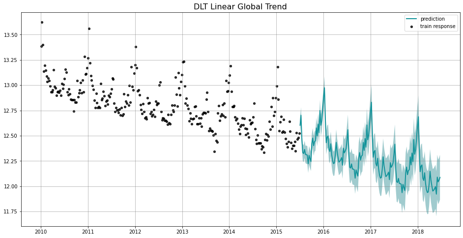
Global Trend Configurations

There are a few choices of \(D(t)\) configured by global_trend_option:

1. loglinear

2. linear

3. flat

4. logistic

To show the difference among these options, we project the predictions in the charts below. Note that the default is set to linear which we find a better fit for a log-transformed model. Such default is also used in the benchmarking process mentioned previously.

%%time
# linear global trend
dlt = DLTMAP(
    response_col=response_col,
    date_col=date_col,
    seasonality=52,
    seed=8888,
)

dlt.fit(train_df)
predicted_df = dlt.predict(test_df)
_ = plot_predicted_data(train_df, predicted_df, date_col, response_col,  title='DLT Linear Global Trend')

CPU times: user 1.4 s, sys: 363 ms, total: 1.76 s
Wall time: 2.02 s

%%time
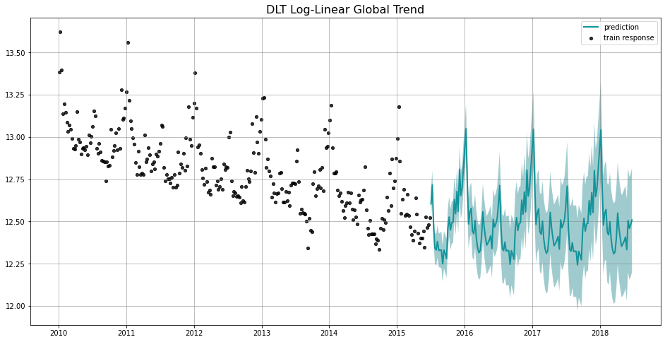
# log-linear global trend
dlt = DLTMAP(
    response_col=response_col,
    date_col=date_col,
    seasonality=52,
    seed=8888,
    global_trend_option='loglinear'
)

dlt.fit(train_df)
predicted_df = dlt.predict(test_df)
_ = plot_predicted_data(train_df, predicted_df, date_col, response_col,  title='DLT Log-Linear Global Trend')

CPU times: user 1.29 s, sys: 292 ms, total: 1.58 s
Wall time: 1.43 s

%%time
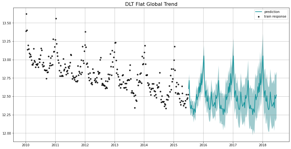
# log-linear global trend
dlt = DLTMAP(
    response_col=response_col,
    date_col=date_col,
    seasonality=52,
    seed=8888,
    global_trend_option='flat'
)

dlt.fit(train_df)
predicted_df = dlt.predict(test_df)
_ = plot_predicted_data(train_df, predicted_df, date_col, response_col,  title='DLT Flat Global Trend')

CPU times: user 1.22 s, sys: 288 ms, total: 1.51 s
Wall time: 1.36 s

%%time
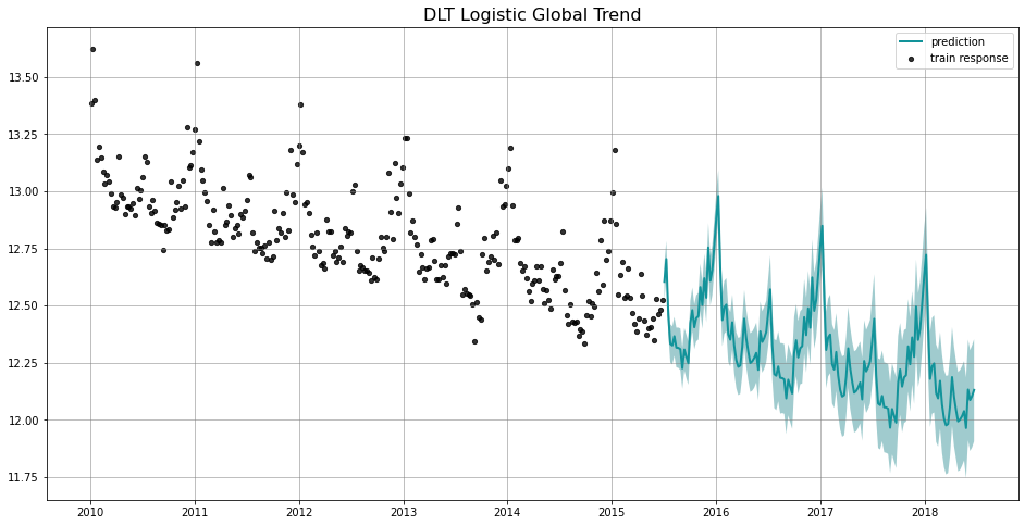
# logistic global trend
dlt = DLTMAP(
    response_col=response_col,
    date_col=date_col,
    seasonality=52,
    seed=8888,
    global_trend_option='logistic'
)

dlt.fit(train_df)
predicted_df = dlt.predict(test_df)
_ = plot_predicted_data(train_df, predicted_df, date_col, response_col,  title='DLT Logistic Global Trend')

CPU times: user 1.36 s, sys: 300 ms, total: 1.66 s
Wall time: 1.54 s

Regression

You can also add regressors into the model by specifying regressor_col. This serves the purpose of nowcasting or forecasting when exogenous regressors are known such as events and holidays. Without losing generality, the interface is set to be

\[\beta_j ~\sim \mathcal{N}(\mu_j, \sigma_j^2)\]

where \(\mu_j = 0\) and \(\sigma_j = 1\) by default as a non-informative prior. These two parameters are set by the arguments regressor_beta_prior and regressor_sigma_prior as a list. For example,

dlt = DLTMAP(
    response_col=response_col,
    date_col=date_col,
    seed=8888,
    seasonality=52,
    regressor_col=['trend.unemploy', 'trend.filling'],
    regressor_beta_prior=[0.1, 0.3],
    regressor_sigma_prior=[0.5, 2.0],
)

dlt.fit(df)
predicted_df = dlt.predict(df, decompose=True)
_ = plot_predicted_components(predicted_df, date_col)

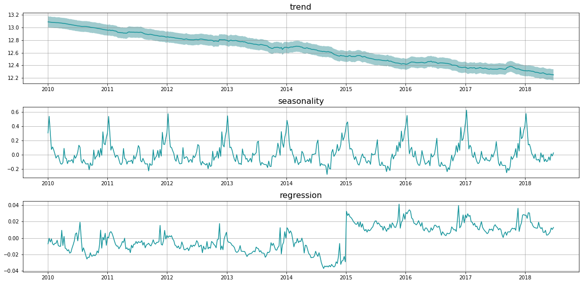
There are much more configurations on regression such as the regressor signs and penalty type. They will be discussed in later section.

Other Configurations

Just like other model, there are full Bayesian version and aggregated posteriors version for DLT named after DLTAggregated and DLTFull. They are usually more robust in regression but may take longer time to train. More details for each method are available in the docstrings and also here: https://uber.github.io/orbit/orbit.models.html#module-orbit.models.dlt